English Premier League Managers

Data Exploration

By Ifeoma Egbogah in Football Bayes R

March 29, 2023

Hi, I'm the here-bot cat!

Use me to find your way in your website.

Here I am:: content/blog/English-Premier-League-Ranking-Series/02-Data-Exploration/Data-Exploration.md

Here is my R Markdown source file:: blog/English-Premier-League-Ranking-Series/02-Data-Exploration/Data-Exploration.Rmd

To remove me, delete this line inside that file: {{< here >}}

My content section is:: blog

My layout is:: single-series

What in the world!!!

I recently came across a post that ranked English Premier League (EPL) managers based on their raw winning percentages. I felt that this approach was unfair to some exceptional managers whose winning averages may not accurately reflect their capabilities due to limited opportunities to manage games. For example, comparing a manager who oversaw 16 wins out of 80 games to one with 70 wins out of 350 games, both with a winning average of 20%, would be unfair.

To address this, I decided to use Bayesian inference to determine the best manager in the Premier League, hoping that it would be Arsene Wenger, as I am a devoted Arsenal fan. Fingers crossed.

As a first step, I loaded the relevant data and packages into R, with the data obtained from the Premier League website (www.premierleague.com). From the league’s inception in 1992 to 2018, a total of 219 managers made their debut in the EPL.

Data

Managers	Clubs	Total Games Managed	Games Won	Games Drawn	Games Lost	Num Of Pl Seasons	Nationality	Date Of Birth	Pl Debut	Debut Match
Eddie Howe	Bournemouth	114	34	30	50	3	England	1977-11-29	2015-08-08	Lost
Brue Rioch	Arsenal	38	17	12	9	1	Scotland	1947-09-06	1995-08-20	Drawn
Arsene Wenger	Arsenal	828	476	199	153	22	France	1949-10-22	1996-10-12	Won
Stewart Houston	Arsenal	19	7	4	8	2	Scotland	1949-08-20	1995-02-21	Won
David O’Leary	Aston Villa	343	148	82	104	7	England	1958-05-02	1998-10-01	na

I spy?

Managers' Age on Debut

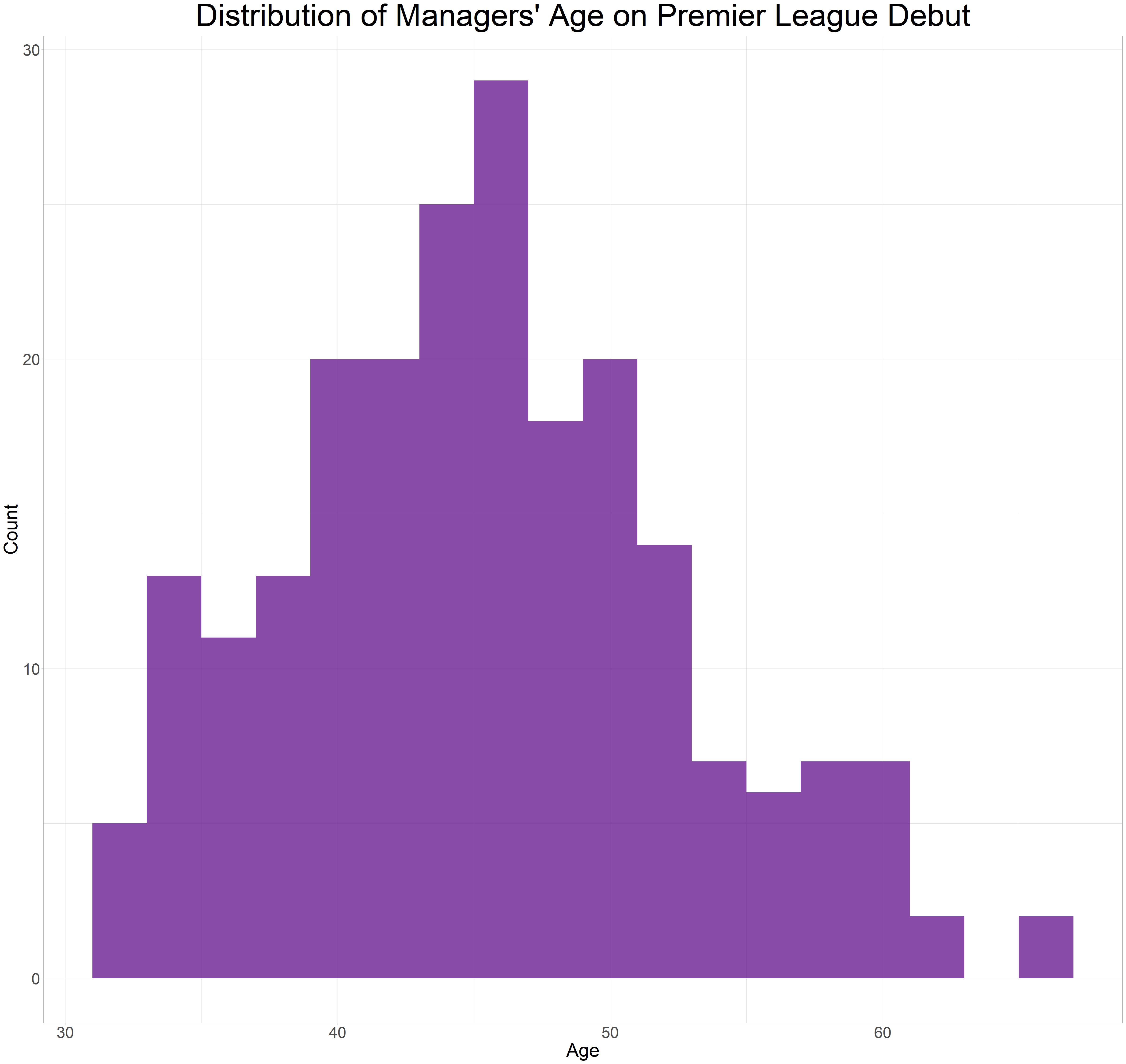
Let’s start by getting to know the data and see what information we can glean from it. This data covers from 1992 to 2018. I begin by calculating the ages of the managers and the mean age at which managers make a debut in the league. The youngest managers in the league were Chris Coleman and Attilio Lombardo while the oldest was Dick Advocaat, making a debut at ages 32 and 67 years respectively. The mean age was 45 years.

Age

Table: Table 1: Youngest and Oldest Managers

Managers	Age
Attilio Lombardo	32
Chris Coleman	32
Dick Advocaat	67

Code

epl <- epl%>%
  mutate(age = year(as.period(interval((date_of_birth), (pl_debut)))))

summary_epl <- epl%>%
  summarise(mean_age = mean(age),
            youngest = min(age),
            oldest = max(age))

age_table <- epl%>%
  select(managers, age)%>%
  filter(age %in% c(32, 67))

knitr::kable(age_table, col.names = c("Managers", "Age"), caption = "Youngest and Oldest Managers")

Table: Table 2: Youngest and Oldest Managers

Managers	Age
Attilio Lombardo	32
Chris Coleman	32
Dick Advocaat	67

Lets get a better view of what the age distribution looks like by plotting a histogram.

Age Distribution

Code

epl%>%
ggplot(aes(age)) + 
  geom_histogram(binwidth = 2, fill = scales::muted("darkorchid"), alpha = 0.8) +
  labs(x = "Age",
      y = "Count",
      title = "Distribution of Managers' Age on Premier League Debut") +
  theme(plot.title = element_text(hjust = 0.5, size = 50),
        axis.title = element_text(size = 30),
        axis.text = element_text(size = 25))

Where are they from?

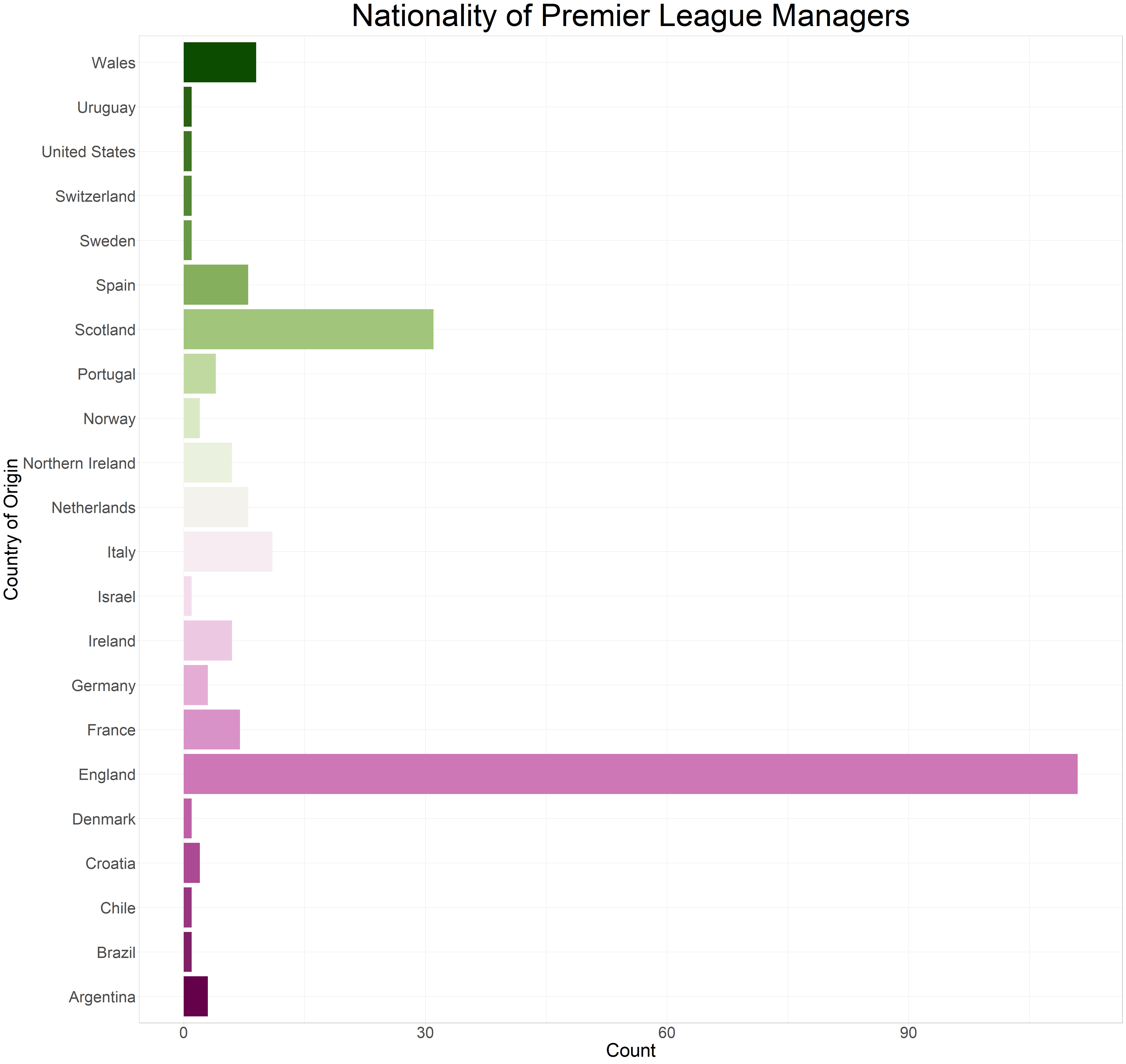
One thing the English League is known for is the wide range in the nationality of not only the players but also the managers of the clubs. So, What is the most common nationality of premier league managers? Let’s find out.

Nationality

Code

epl %>%
  count(nationality, sort=TRUE) %>%
 # mutate(nationality = fct_reorder(nationality, n))%>%
  ggplot(aes(nationality, n)) + 
  geom_col(aes(fill = nationality)) + 
  labs(x = "Country of Origin",
       y = "Count", 
       title = "Nationality of Premier League Managers") +
  scale_fill_scico_d(palette = "bam") +
  theme(legend.position = "none",
        plot.title = element_text(hjust = 0.5, size = 50),
        axis.title = element_text(size = 30),
        axis.text = element_text(size = 25)) + 
  coord_flip()

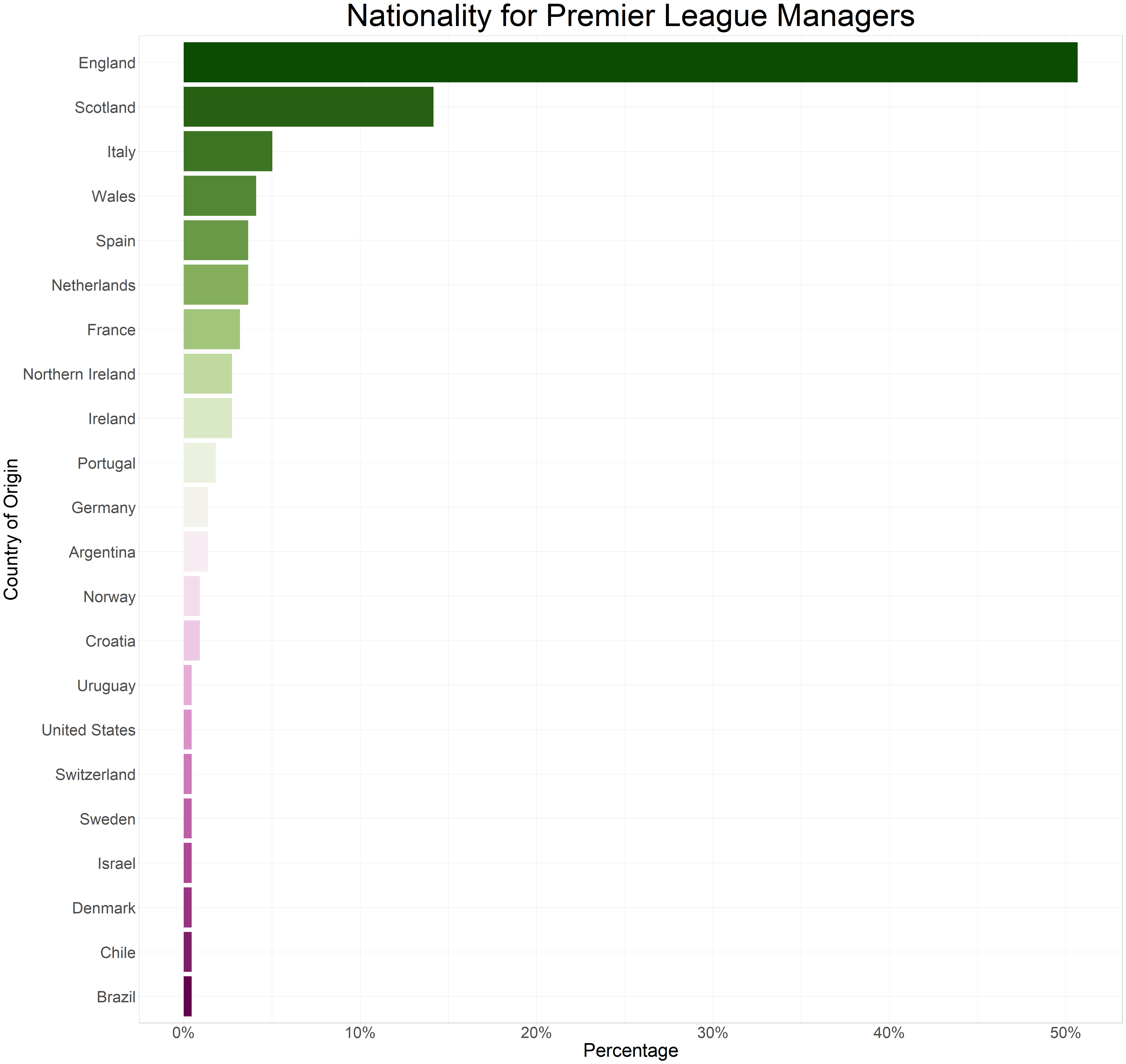
Err… it looks a bit scattered let’s arrange it in descending order based on there percentage so as to get a clearer picture.

Nationality Arranged

Code

Origin <- epl%>%
  count(nationality, sort=TRUE) %>%
  mutate(percent = (n/sum(n))) %>%
  mutate(country = fct_reorder(nationality, percent))%>%
  ggplot(aes(country, percent)) + 
  geom_col(aes(fill = country)) + 
  labs(x = "Country of Origin",
       y = "Percentage",
       title = "Nationality for Premier League Managers") +
  scale_fill_scico_d(palette = "bam") +
  scale_y_continuous(labels = label_percent()) +
  theme(legend.position = "none",
        plot.title = element_text(hjust = 0.5, size = 50),
        axis.title = element_text(size = 30),
        axis.text = element_text(size = 25)) +
  coord_flip()


Origin

That’s much better. Here we can see that most managers in the league are English with 51%, followed by the Scots at 13%. Uruguay, United States, Switzerland, Sweden, Israel, Denmark, Chile and Brazil have each had one manager from these countries debuting in the premier league.

Who Runs the Top Flight Clubs?

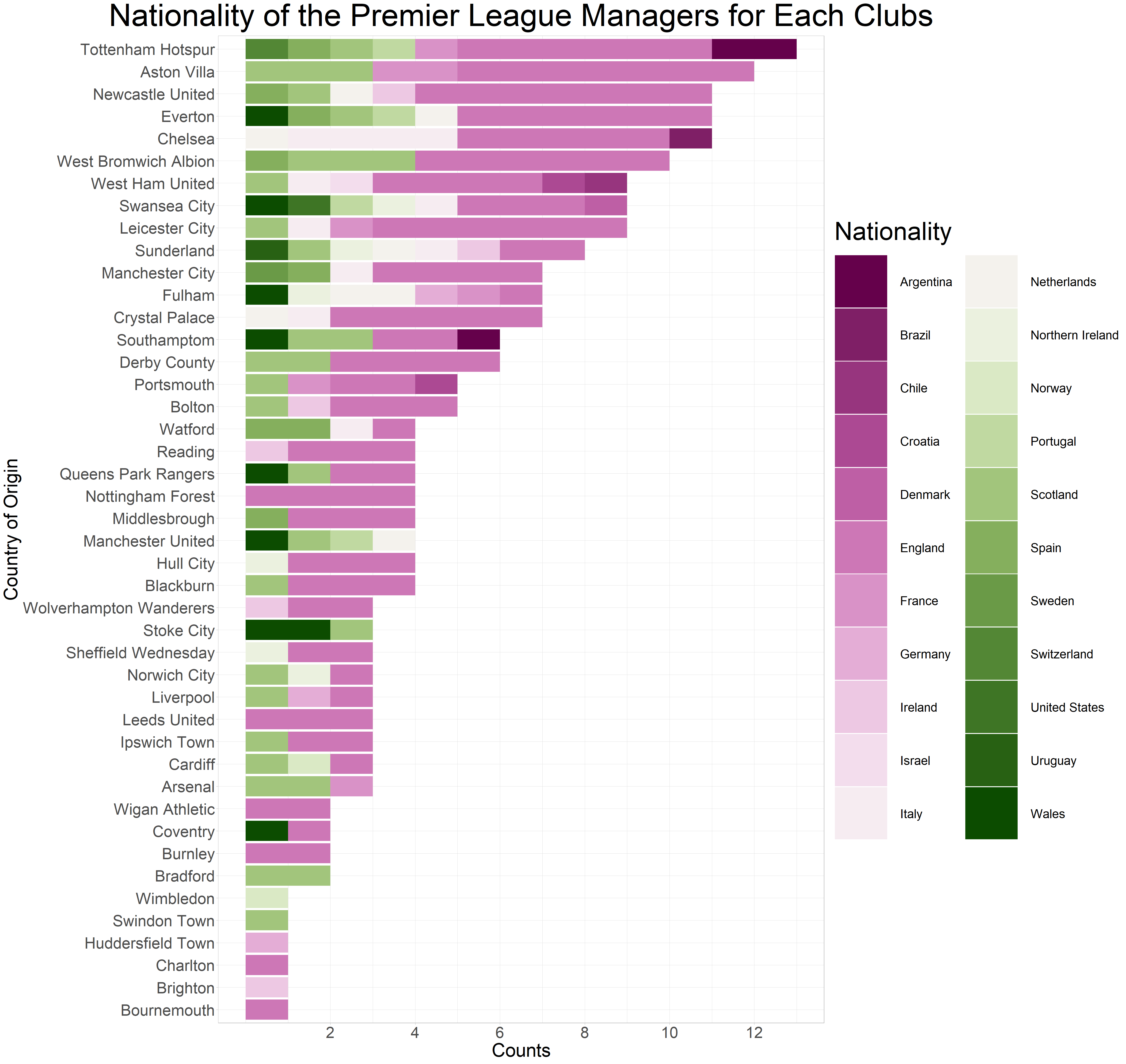
A popular opinion among sports pundits is that English managers haven’t been given the chance to over see the top flight clubs in the league. How true is this? Let’s find out.

Club

Code

all_club <- epl%>%
  count(nationality, clubs, sort = TRUE)%>%
  group_by(clubs)%>%
  mutate(total = sum(n))%>%
  ggplot(aes(fct_reorder(clubs, total), n)) + 
  geom_col(aes(fill= nationality)) +
  labs(x = "Country of Origin",
       y = "Counts",
       fill = "Nationality",
       title = "Nationality of the Premier League Managers for Each Clubs") +
  scale_fill_scico_d(palette = "bam") +
  scale_y_continuous(breaks = seq(2, 12, 2)) +
  coord_flip() +
  theme(plot.title = element_text(hjust = 0.5, size = 50),
        axis.title = element_text(size = 30),
        axis.text = element_text(size = 25),
        legend.title = element_text(size = 40),
        legend.key.size  = unit(3, "cm"),
        legend.text = element_text(size = 20))



top_club <- epl%>%
  filter(clubs %in% c("Arsenal", "Chelsea", "Manchester United", "Manchester City", "Liverpool", "Tottenham Hotspur"))%>%
  count(nationality, clubs, sort = TRUE)%>%
  group_by(clubs)%>%
  mutate(total = sum(n))%>%
  ggplot(aes(fct_reorder(clubs, total), n)) + 
  geom_col(aes(fill= nationality)) +
  labs(x = "Country of Origin",
       y = "Counts",
       fill = "Nationality",
       title = "Nationality of the Premier League Managers for the Top Flight Clubs") +
  scale_fill_scico_d(palette = "bam") +
  scale_y_continuous(breaks = seq(2, 12, 2)) +
  coord_flip() +
  theme(plot.title = element_text(hjust = 0.5, size = 40),
        axis.title = element_text(size = 30),
        axis.text = element_text(size = 22),
        legend.title = element_text(size = 35),
        legend.key.size  = unit(2, "cm"),
        legend.text = element_text(size = 25))

all_club

top_club

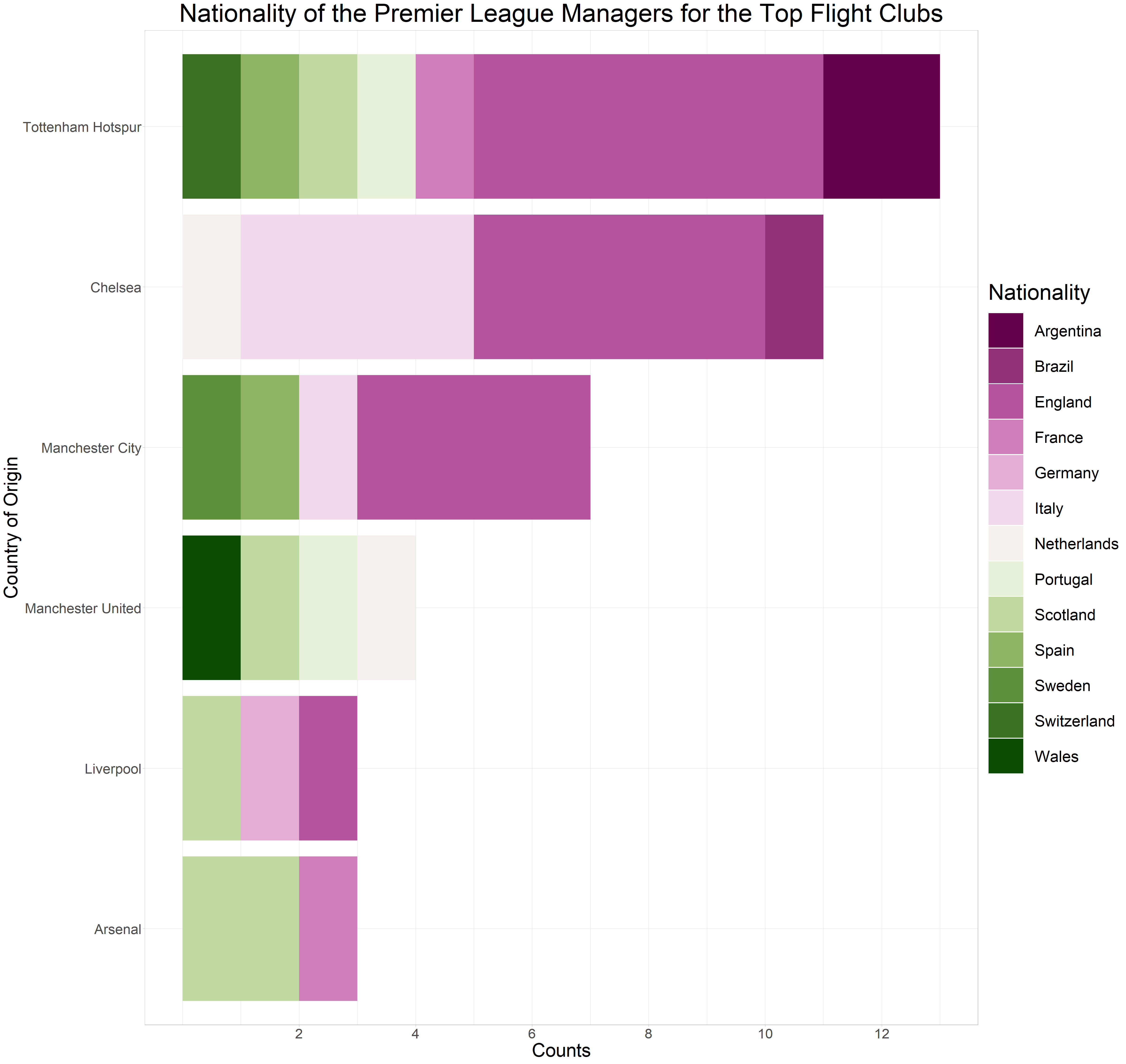
The bar chart above shows that all the top 6 clubs except Manchester United and Arsenal have had an English Manager in charge. Manchester united not having an English manager since the creation of the league is partially because Sir Alex Ferguson (who debuted at the club in 1986) was the manager of the club before the league was created and he spent over 20 years at the helm of affairs in the club before handing over at the end of 2012/13 season.

Match Result on Premier League Debut

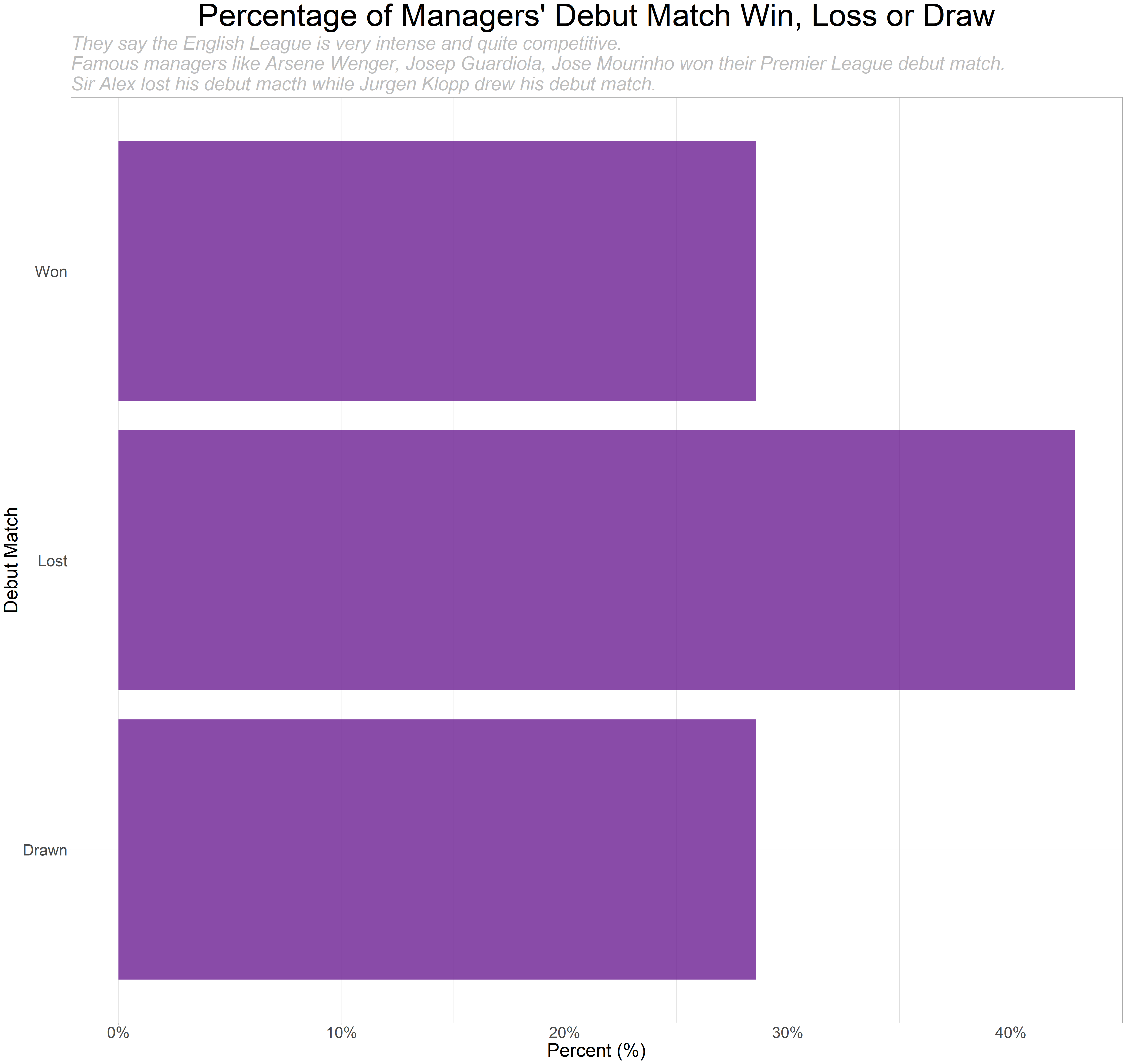
David O’Leary and Martin O’Neill had no information on their English premier league debut. So I’ll filter them out. Most managers lost on their first English premier league debut (42.5%).

Match Result

Code

debut <- epl %>%
  filter(debut_match != "na") %>%
  count(debut_match, sort=TRUE) %>%
  mutate(percent = (n/sum(n)))%>%
  ggplot(aes(percent, debut_match)) +
  geom_col(fill = scales::muted("darkorchid"), alpha = 0.8) +
  scale_x_continuous(labels = scales::label_percent())+
  labs(x = "Percent (%)",
       y = "Debut Match",
       title = "Percentage of Managers' Debut Match Win, Loss or Draw",
       subtitle = "They say the English League is very intense and quite competitive.\nFamous managers like Arsene Wenger, Josep Guardiola, Jose Mourinho won their Premier League debut match.\nSir Alex lost his debut macth while Jurgen Klopp drew his debut match.") +
  theme(plot.title = element_text(hjust = 0.5, size = 50),
        plot.subtitle = element_text(face = "italic", size = 30, colour = "grey"),
        legend.text = element_text(size = 15),
        axis.title = element_text(size = 30),
        axis.text = element_text(size = 25))

debut

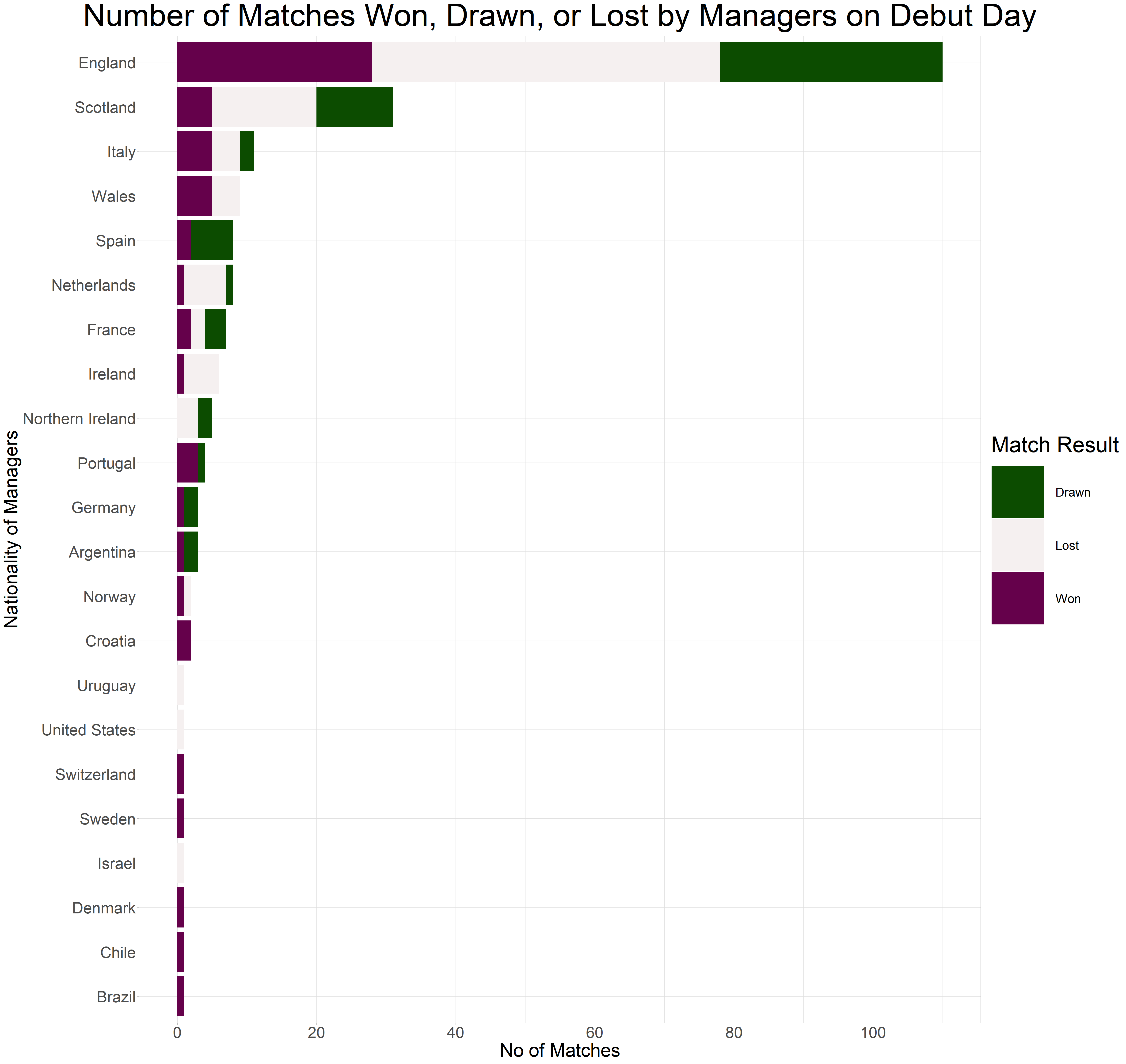
Out of the 112 English managers in the league 50 lost their debut matches. So far no Argentine, German, Portuguese or Spanish managers have lost their debut match.

Debut Result by Nationality

Code

debut_nat <- epl %>%
  filter(debut_match != "na") %>%
  count(debut_match, nationality, sort=TRUE)%>%
  group_by(nationality)%>%
  mutate(total = sum(n))%>%
  ggplot(aes(fct_reorder(nationality, total), n)) + 
  geom_col(aes(fill = debut_match)) +
  coord_flip() +
  scale_fill_scico_d(palette = "bam", direction = -1) +
  scale_y_continuous(breaks = seq(0, 130, 20)) +
  labs(x = "Nationality of Managers",
       y = "No of Matches",
       title = "Number of Matches Won, Drawn, or Lost by Managers on Debut Day",
       fill = "Match Result") +
  theme(plot.title = element_text(hjust = 0.5, size = 50),
        axis.title = element_text(size = 30),
        axis.text = element_text(size = 25),
        legend.title = element_text(size = 35),
        legend.key.size  = unit(3, "cm"),
        legend.text = element_text(size = 20))

debut_nat

Out of the 112 English managers in the league 50 lost their debut matches. So far no Argentine, German, Portuguese or Spanish managers have lost their debut match.

Now that we have explored our data, we will begin analyzing in the next post.