English Premier League Managers
The Best and Worst EPL Managers Using Emprirical Bayes
By Ifeoma Egbogah in Football Bayes R
April 17, 2023
Introduction
In the last post I mentioned I read an article where the English Premier League managers' were ranked based on their raw winning averages. I felt this was a bit unfair. In this post I am going to attempt to rank each managers' performance in the premier league using the Empirical Bayes method to estimate their winning average as against using their raw winning averages and the manager with the highest average is our best manager.This borrows from Dave’s post on “Understanding Empirical Bayes Estimation Using Baseball Statistics”. (http://varianceexplained.org/). It is a great read.
So we are going to use the empirical Bayes method to: ** estimate the winning average of each manager ** estimate their credible interval
Let’s load our data set (data used in the Data-Exploration blog post (https://ifeoma-egbogah.netlify.app/blog/english-premier-league-ranking-series/02-data-exploration/data-exploration/)) and packages into R.
Raw Winning Average
The primary measure of a manager’s performance is the outcome of the matches under their charge, which can result in a win, draw, or loss. When victory appears unlikely, managers tend to prefer a draw over a loss, as the team would earn a point instead of none. Winning a match rewards the team with three points.
So, who are the best and worst managers? Let’s find out…..
Raw Winning Average = Games Won/Total Games Managed
These are the ten managers with the highest raw winning average.
| Managers | Total Games Managed | Games Won | Games Drawn | Games Lost | Average |
|---|---|---|---|---|---|
| Jim Barron | 1 | 1 | 0 | 0 | 1.000 |
| Eddie Newton | 1 | 1 | 0 | 0 | 1.000 |
| Josep Guardiola | 76 | 55 | 13 | 8 | 0.724 |
| Antonio Conte | 76 | 51 | 10 | 15 | 0.671 |
| Trevor Brooking | 3 | 2 | 1 | 0 | 0.667 |
| Alex Ferguson | 810 | 528 | 168 | 114 | 0.652 |
| Jose Mourinho | 288 | 183 | 65 | 40 | 0.635 |
| Carlo Ancelotti | 76 | 48 | 13 | 15 | 0.632 |
| Roberto Mancini | 133 | 82 | 27 | 24 | 0.617 |
| Manuel Pellegrini | 114 | 70 | 21 | 23 | 0.614 |
rwa_top <- epl %>%
  arrange(desc(average)) %>%
  dplyr::select(managers, total_games_managed, games_won, games_drawn, games_lost, average) %>%
  head(10)


knitr::kable(rwa_top, col.names = str_to_title(str_replace_all(names(rwa_top), "_", " ")))
| Managers | Total Games Managed | Games Won | Games Drawn | Games Lost | Average |
|---|---|---|---|---|---|
| Jim Barron | 1 | 1 | 0 | 0 | 1.000 |
| Eddie Newton | 1 | 1 | 0 | 0 | 1.000 |
| Josep Guardiola | 76 | 55 | 13 | 8 | 0.724 |
| Antonio Conte | 76 | 51 | 10 | 15 | 0.671 |
| Trevor Brooking | 3 | 2 | 1 | 0 | 0.667 |
| Alex Ferguson | 810 | 528 | 168 | 114 | 0.652 |
| Jose Mourinho | 288 | 183 | 65 | 40 | 0.635 |
| Carlo Ancelotti | 76 | 48 | 13 | 15 | 0.632 |
| Roberto Mancini | 133 | 82 | 27 | 24 | 0.617 |
| Manuel Pellegrini | 114 | 70 | 21 | 23 | 0.614 |
…..and these are the ten managers with lowest raw winning average.
| Managers | Total Games Managed | Games Won | Games Drawn | Games Lost | Average |
|---|---|---|---|---|---|
| Eric Black | 9 | 0 | 1 | 8 | 0 |
| Archie Knox | 1 | 0 | 0 | 1 | 0 |
| Staurt McCall | 2 | 0 | 0 | 2 | 0 |
| Steve Holland | 1 | 0 | 0 | 1 | 0 |
| Frank de Boer | 4 | 0 | 0 | 4 | 0 |
| Billy McEwan | 1 | 0 | 0 | 1 | 0 |
| Jimmy Gabriel | 7 | 0 | 1 | 6 | 0 |
| Ray Lewington | 3 | 0 | 2 | 1 | 0 |
| Paul Goddard | 2 | 0 | 2 | 1 | 0 |
| Tony Book | 1 | 0 | 1 | 0 | 0 |
rwa_bottom <- epl %>%
  arrange(average) %>%
  dplyr::select(managers, total_games_managed, games_won, games_drawn, games_lost, average) %>%
  head(10)


knitr::kable(rwa_bottom, col.names = str_to_title(str_replace_all(names(rwa_bottom), "_", " ")))
| Managers | Total Games Managed | Games Won | Games Drawn | Games Lost | Average |
|---|---|---|---|---|---|
| Eric Black | 9 | 0 | 1 | 8 | 0 |
| Archie Knox | 1 | 0 | 0 | 1 | 0 |
| Staurt McCall | 2 | 0 | 0 | 2 | 0 |
| Steve Holland | 1 | 0 | 0 | 1 | 0 |
| Frank de Boer | 4 | 0 | 0 | 4 | 0 |
| Billy McEwan | 1 | 0 | 0 | 1 | 0 |
| Jimmy Gabriel | 7 | 0 | 1 | 6 | 0 |
| Ray Lewington | 3 | 0 | 2 | 1 | 0 |
| Paul Goddard | 2 | 0 | 2 | 1 | 0 |
| Tony Book | 1 | 0 | 1 | 0 | 0 |
Wow, isn’t this interesting. Observing the table, we can conclude that these managers are neither the best nor the worst in the league. The raw winning averages are therefore not a reliable indicator for identifying the best and worst managers in the league. This measure only takes into account managers who have led a single game and happened to be either ‘lucky’ or ‘unlucky’ in winning or losing the match.
The average raw winning percentage across all managers is 0.282.
We definitely need a better estimate. Let’s get it.
Distribution of the Raw Winning Average
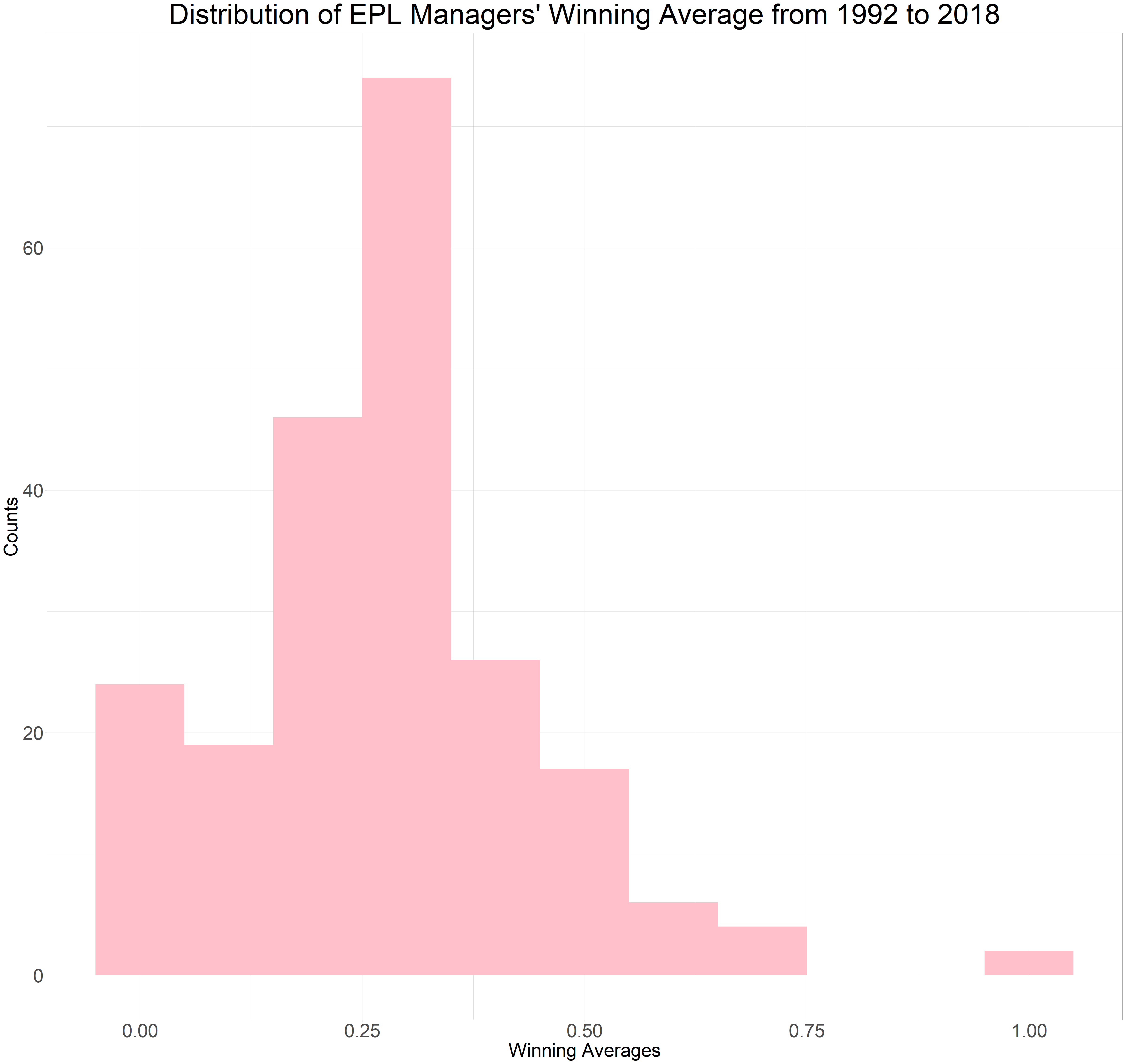
To start, we will analyze the raw winning averages of the managers by observing their distribution, typically accomplished by creating a histogram. After reviewing the histogram, we can conclude that the beta distribution is a suitable option for both our prior distribution and our binomial data.
epl%>%
  dplyr::select(managers, total_games_managed, games_won, games_drawn, games_lost)%>%
  mutate(average = games_won/total_games_managed)%>%
  ggplot(aes(average)) +
  geom_histogram(binwidth = 0.1, fill="pink") +
  labs(x = "Winning Averages",
       y = "Counts",
       title = "Distribution of EPL Managers' Winning Average from 1992 to 2018") +
  theme_light() +
  theme(plot.title = element_text(hjust = 0.5, size = 45),
        axis.title = element_text(size = 30),
        axis.text = element_text(size = 30))
What is Bayesian Inference?
Bayes typically refers to Thomas Bayes, an 18th-century British mathematician and theologian who developed Bayes' theorem, a fundamental concept in Bayesian inference. Bayes' theorem is a mathematical formula that describes the probability of an event based on prior knowledge or beliefs about the event and new evidence or data. Bayesian inference is a statistical approach that uses Bayes' theorem to update probabilities and make predictions based on new data or evidence
Empirical Bayes
Empirical Bayes is a statistical approach that combines frequentist and Bayesian methods to estimate the parameters of a statistical model. Empirical Bayes methods use a two-stage process to estimate parameters: first, they estimate the prior distribution of the parameters based on observed data, and then they use Bayesian methods to estimate the posterior distribution.
The key idea behind empirical Bayes is to estimate the prior distribution of the parameters based on the same data that is used to estimate the parameters themselves. This approach is useful when there is not enough data to estimate the prior distribution independently, or when the prior distribution is too broad and uninformative. By using the observed data to estimate the prior distribution, the empirical Bayes approach can often provide more accurate parameter estimates than standard frequentist methods.
Empirical Bayes methods have been widely used in many applications, including sports analytics, genomics, and economics. In sports analytics, empirical Bayes is used to estimate the performance of players based on their past performance and the performance of their opponents. In genomics, it is used to estimate the expression of genes based on DNA microarray data. In economics, it is used to estimate the impact of policies or programs on outcomes such as employment or income.
Step 1: Prior Distribution
The initial stage of Bayesian analysis involves selecting a prior distribution, which, in the case of empirical Bayes, is derived from the data. While this approach may not adhere strictly to Bayesian principles, I opted for it as I had a substantial amount of data available. Thus, our model takes the form of:
$$Y\sim\mbox{Binomial} (Total\ Games\ Managed,\ X)$$
$$X\sim\mbox{Beta}(\alpha,\ \beta)$$
The “hyper parameters” of our model are denoted by $$\alpha$$ and $$\beta$$. To determine these hyper parameters, we will employ the method of moments or maximum likelihood estimation. In this instance, we will be utilizing the method of moments, which involves calculating the mean and variance of the data. The formula for the method of moments is as follows:
$$\mu\ = mean(X)$$
$$\sigma\ = var(X)$$
$$\alpha = ((1 - \mu)/\sigma - 1/\mu) * \mu^2$$
$$\beta = \alpha * (1 /\mu -1 )$$
The fitdist function from the fitdistrplus package can be used to calculate the method of moments. I filtered out the total games managed that were less than 10 to reduce the noise. This gives us $$\alpha$$ = 3.77, $$\beta$$ = 8.631.
## Fitting of the distribution ' beta ' by matching moments
## Parameters :
##        estimate
## shape1     3.77
## shape2     8.63
## Loglikelihood:  -Inf   AIC:  Inf   BIC:  Inf
## shape1
##   3.77
## shape2
##   8.63
epl_man <- epl %>%
  filter(total_games_managed >= 10)


e <- fitdist(epl_man$average, "beta", method="mme")

summary(e)
## Fitting of the distribution ' beta ' by matching moments
## Parameters :
##        estimate
## shape1     3.77
## shape2     8.63
## Loglikelihood:  -Inf   AIC:  Inf   BIC:  Inf
alpha <- e$estimate[1]
beta <- e$estimate[2]

alpha
## shape1
##   3.77
beta
## shape2
##   8.63
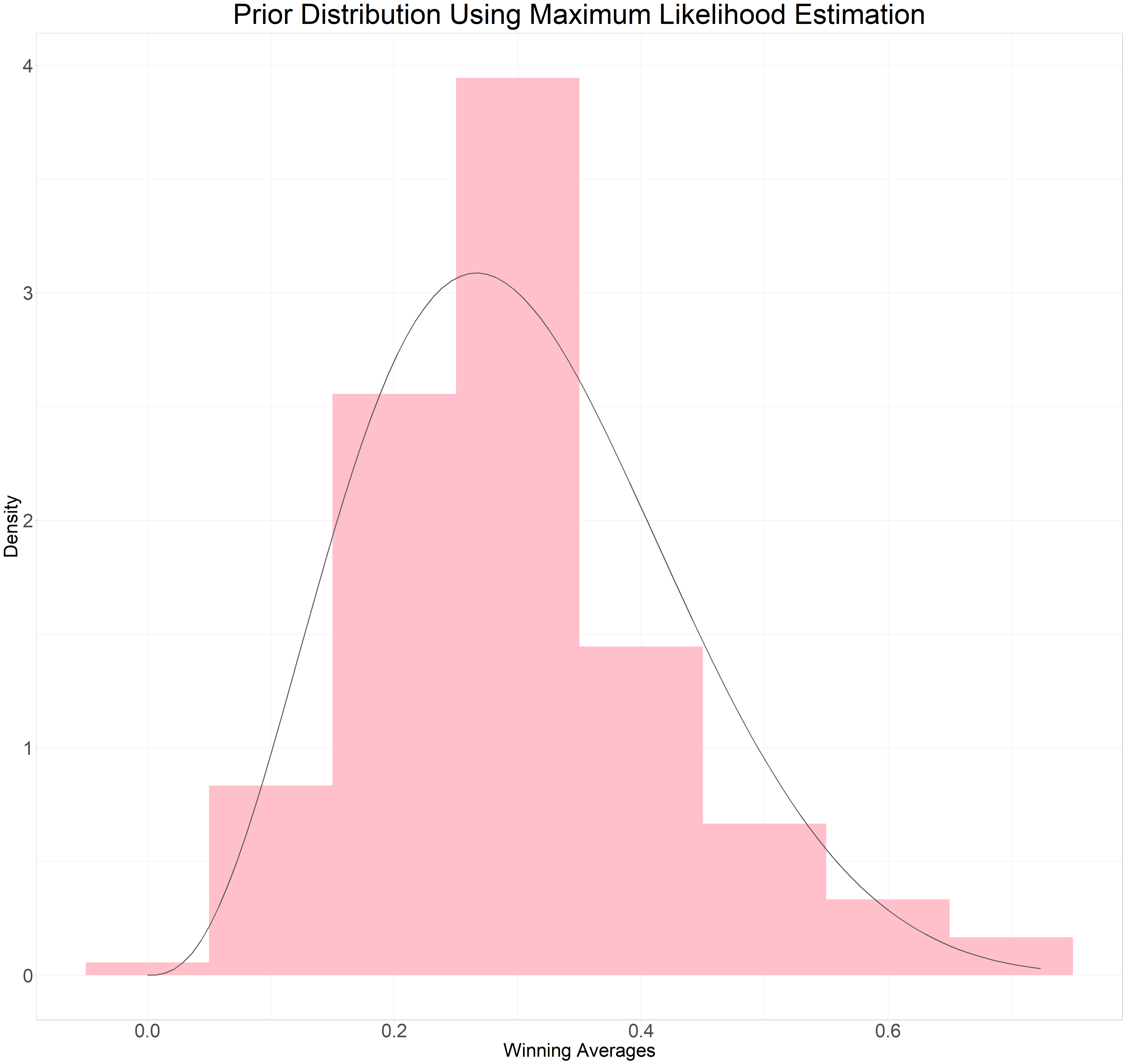
We can visualize the fit of the shape parameters for the beta distribution to the distribution of the raw winning averages shown in the histogram by plotting the distribution and examining its alignment
epl_man%>%
  ggplot() +
  geom_histogram(aes(average, y = after_stat(density)), binwidth=0.1, fill = "pink") +
  stat_function(fun = function(x) dbeta(x, alpha, beta), colour="grey35", linewidth = 0.8) +
  labs(x = "Winning Averages",
  y = "Density",
  title = "Prior Distribution Using Maximum Likelihood Estimation") +
  theme_light() +
  theme(plot.title = element_text(hjust = 0.5, size = 45),
        axis.title = element_text(size = 30),
        axis.text = element_text(size = 30))
Not perfect but not to bad. Next stop empirical Bayes estimate, then posterior probability and finally credible interval.
Step 2: Applying the Beta Distribution as a Prior for the Winning Average of Each Manager.
Since we have our prior probability distribution we can now calculate our posterior winning average for each manager by updating based on individual evidence. We do this by:
$$Posterior\ Winning\ Estimate = \frac{\alpha + Games\ Won}{\alpha + \beta + Total\ Games\ Managed}$$
Simple right.
| Managers | Average | Eb Winning Average |
|---|---|---|
| Eddie Howe | 0.298 | 0.299 |
| Brue Rioch | 0.447 | 0.412 |
| Arsene Wenger | 0.575 | 0.571 |
| Stewart Houston | 0.368 | 0.343 |
| David O’Leary | 0.431 | 0.427 |
| Jim Barron | 1.000 | 0.356 |
| Tim Sherwood | 0.422 | 0.397 |
| Graham Taylor | 0.236 | 0.244 |
| Brian Little | 0.368 | 0.363 |
| Remi Garde | 0.100 | 0.178 |
epl <-epl %>%
  mutate(eb_winning_average = (games_won + alpha)/(total_games_managed + alpha + beta))


epl%>%
  dplyr::select(managers, average, eb_winning_average)%>%
  head(10)%>%
  knitr::kable(col.names = str_to_title(str_replace_all(names(.), "_", " ")))
| Managers | Average | Eb Winning Average |
|---|---|---|
| Eddie Howe | 0.298 | 0.299 |
| Brue Rioch | 0.447 | 0.412 |
| Arsene Wenger | 0.575 | 0.571 |
| Stewart Houston | 0.368 | 0.343 |
| David O’Leary | 0.431 | 0.427 |
| Jim Barron | 1.000 | 0.356 |
| Tim Sherwood | 0.422 | 0.397 |
| Graham Taylor | 0.236 | 0.244 |
| Brian Little | 0.368 | 0.363 |
| Remi Garde | 0.100 | 0.178 |
Results
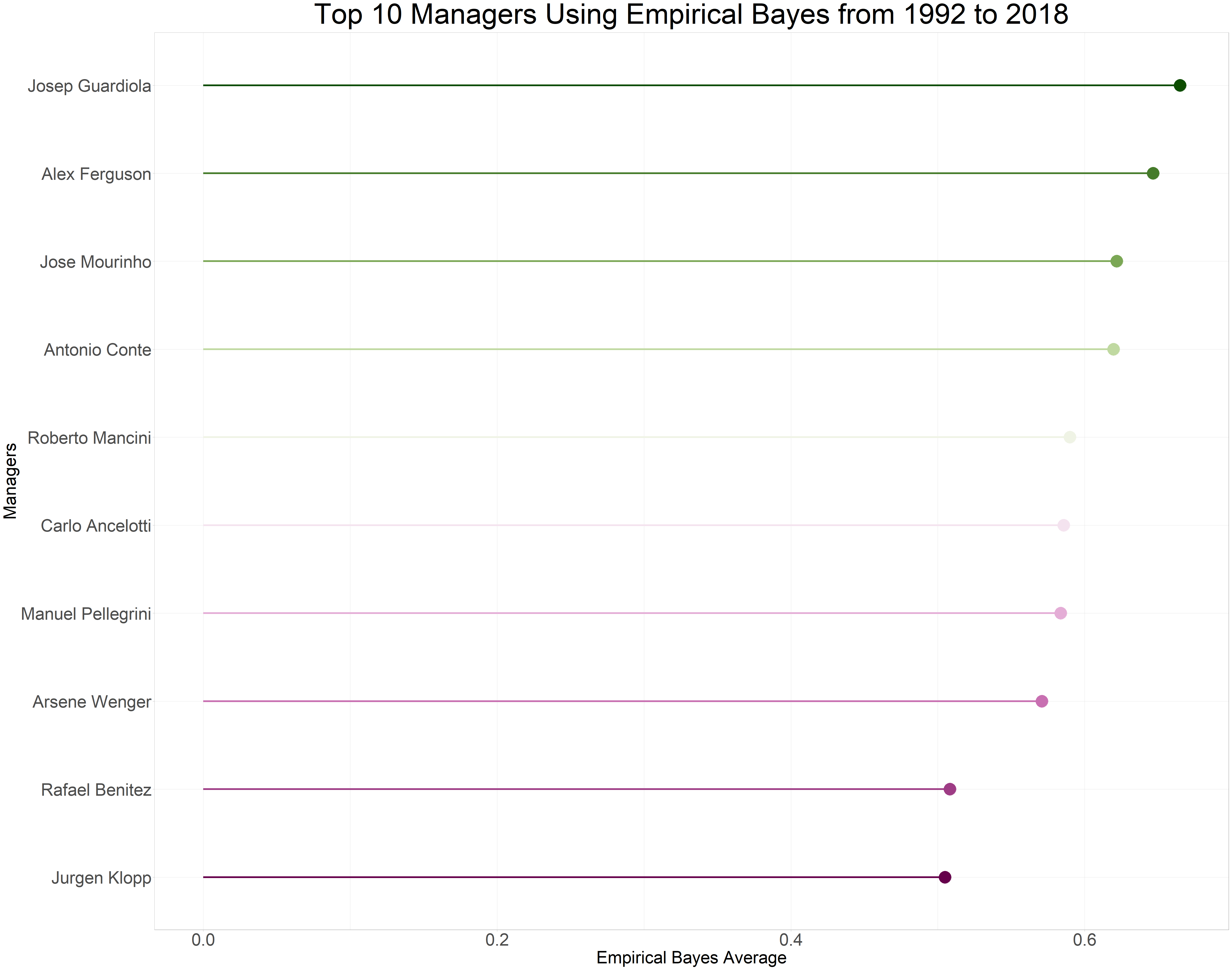
According to this estimate, the top ten managers are in! Drum roll, please. And the winner is Pep Josep Guadiola with a remarkable winning average of 0.665 (66.5%), even though he has only spent two seasons in the league based on this data. Coming in at a close second is Alex Ferguson with a winning average of 0.647 (64.7%). Another notable mention goes to the Prof (Arsene Wenger), who secures the number 8 spot with a winning average of 0.571 (57.10%).
| Managers | Total Games Managed | Games Won | Average | Eb Winning Average |
|---|---|---|---|---|
| Josep Guardiola | 76 | 55 | 0.724 | 0.665 |
| Alex Ferguson | 810 | 528 | 0.652 | 0.647 |
| Jose Mourinho | 288 | 183 | 0.635 | 0.622 |
| Antonio Conte | 76 | 51 | 0.671 | 0.620 |
| Roberto Mancini | 133 | 82 | 0.617 | 0.590 |
| Carlo Ancelotti | 76 | 48 | 0.632 | 0.586 |
| Manuel Pellegrini | 114 | 70 | 0.614 | 0.584 |
| Arsene Wenger | 828 | 476 | 0.575 | 0.571 |
| Rafael Benitez | 302 | 156 | 0.517 | 0.508 |
| Jurgen Klopp | 106 | 56 | 0.528 | 0.505 |
epl_man2 <- epl %>%
  arrange(desc(eb_winning_average)) %>%
  dplyr::select(managers, total_games_managed, games_won, average, eb_winning_average) %>%
  head(10)

knitr::kable(epl_man2, col.names = str_to_title(str_replace_all(names(epl_man2), "_", " ")))
| Managers | Total Games Managed | Games Won | Average | Eb Winning Average |
|---|---|---|---|---|
| Josep Guardiola | 76 | 55 | 0.724 | 0.665 |
| Alex Ferguson | 810 | 528 | 0.652 | 0.647 |
| Jose Mourinho | 288 | 183 | 0.635 | 0.622 |
| Antonio Conte | 76 | 51 | 0.671 | 0.620 |
| Roberto Mancini | 133 | 82 | 0.617 | 0.590 |
| Carlo Ancelotti | 76 | 48 | 0.632 | 0.586 |
| Manuel Pellegrini | 114 | 70 | 0.614 | 0.584 |
| Arsene Wenger | 828 | 476 | 0.575 | 0.571 |
| Rafael Benitez | 302 | 156 | 0.517 | 0.508 |
| Jurgen Klopp | 106 | 56 | 0.528 | 0.505 |
epl %>%
  arrange(desc(eb_winning_average)) %>%
  dplyr::select(managers, total_games_managed, games_won, average, eb_winning_average) %>%
  head(10)%>%
  mutate(managers = fct_reorder(managers, eb_winning_average))%>%
  ggplot(aes(eb_winning_average, managers, colour = managers)) +
  geom_point(show.legend = FALSE, size = 10) +
  geom_segment(aes(xend = 0, yend = managers), linewidth = 1.5, show.legend = FALSE) +
  scale_color_scico_d(palette = "bam") +
  labs(x = "Empirical Bayes Average",
       y = "Managers",
       title = "Top 10 Managers Using Empirical Bayes from 1992 to 2018") +
  theme_light() +
  theme(plot.title = element_text(hjust = 0.5, size = 50),
        axis.title = element_text(size = 30),
        axis.text = element_text(size = 30))
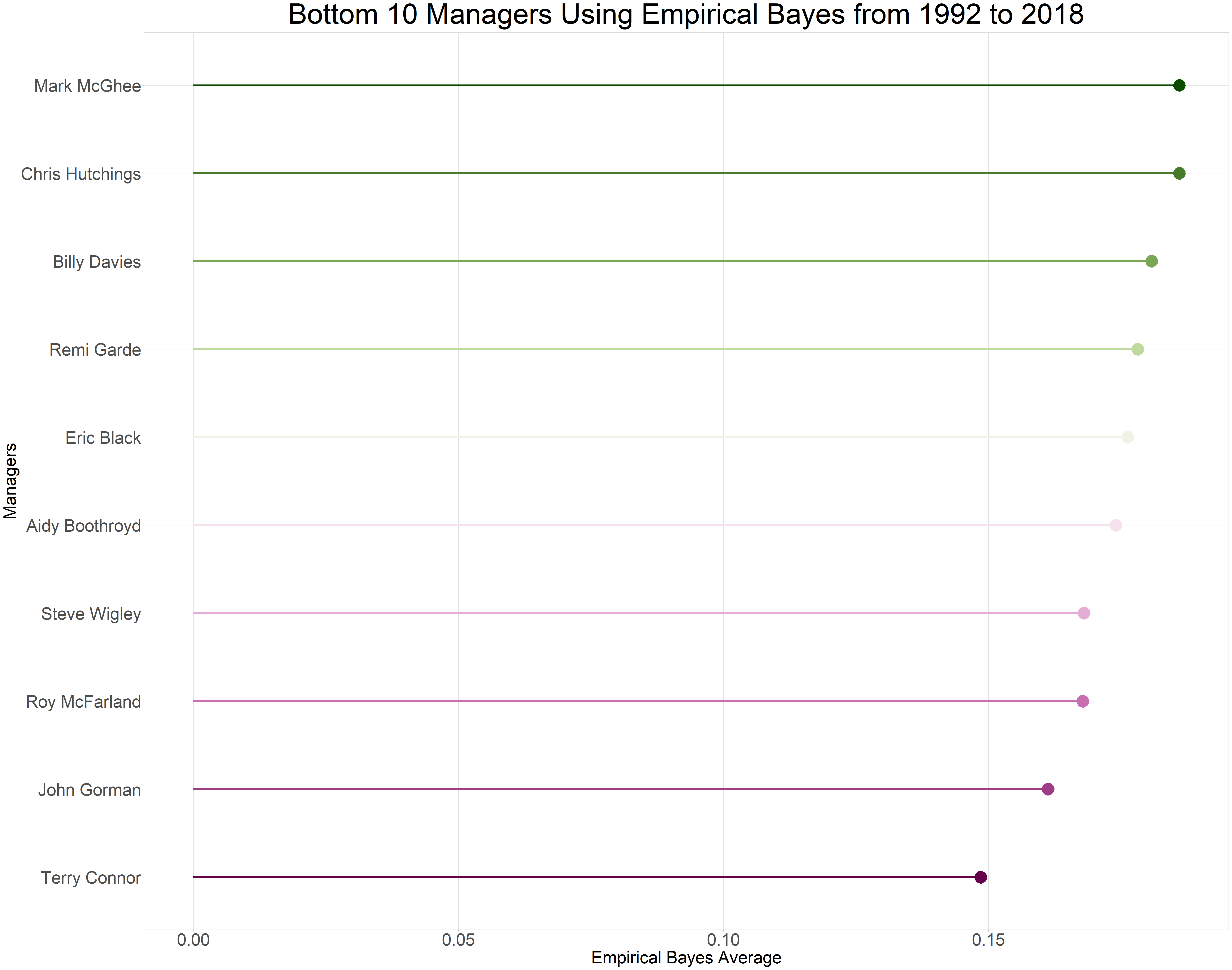
Let’s move on to the bottom ten managers in the Premier League based on our estimates. According to the data, Terry Connor had the lowest winning average of 0.1504 (15.04%). Interestingly, we can observe that the empirical Bayes estimation did not include managers who only managed one or two games, unlike the raw winning average.
| Managers | Total Games Managed | Games Won | Average | Eb Winning Average |
|---|---|---|---|---|
| Terry Connor | 13 | 0 | 0.000 | 0.149 |
| John Gorman | 42 | 5 | 0.119 | 0.161 |
| Roy McFarland | 22 | 2 | 0.091 | 0.168 |
| Steve Wigley | 16 | 1 | 0.062 | 0.168 |
| Aidy Boothroyd | 38 | 5 | 0.132 | 0.174 |
| Eric Black | 9 | 0 | 0.000 | 0.176 |
| Remi Garde | 20 | 2 | 0.100 | 0.178 |
| Billy Davies | 14 | 1 | 0.071 | 0.181 |
| Mark McGhee | 24 | 3 | 0.125 | 0.186 |
| Chris Hutchings | 24 | 3 | 0.125 | 0.186 |
epl %>%
  arrange(eb_winning_average) %>%
  dplyr::select(managers, total_games_managed, games_won, average, eb_winning_average) %>%
  head(10)%>%
  mutate(managers = fct_reorder(managers, eb_winning_average))%>%
  ggplot(aes(eb_winning_average, managers, colour = managers)) +
  geom_point(show.legend = FALSE, size = 10) +
  geom_segment(aes(xend = 0, yend = managers), linewidth = 1.5, show.legend = FALSE) +
  scale_color_scico_d(palette = "bam") +
  labs(x = "Empirical Bayes Average",
       y = "Managers",
       title = "Bottom 10 Managers Using Empirical Bayes from 1992 to 2018") +
  theme_light() +
  theme(plot.title = element_text(hjust = 0.5, size = 50),
        axis.title = element_text(size = 30),
        axis.text = element_text(size = 30))
Posterior Distribution
Now that we have obtained our posterior winning average, it is possible to determine the shape parameters of the posterior probability distribution for each manager. Updating the shape parameters of the prior beta distribution can achieve this with ease.
| Managers | Alpha2 | Beta2 |
|---|---|---|
| Eddie Howe | 37.77 | 88.63 |
| Brue Rioch | 20.77 | 29.63 |
| Arsene Wenger | 479.77 | 360.63 |
| Stewart Houston | 10.77 | 20.63 |
| David O’Leary | 151.77 | 203.63 |
| Jim Barron | 4.77 | 8.63 |
| Tim Sherwood | 22.77 | 34.63 |
| Graham Taylor | 24.77 | 76.63 |
| Brian Little | 56.77 | 99.63 |
| Remi Garde | 5.77 | 26.63 |
epl <- epl%>%
  mutate(alpha2 = games_won + alpha,
         beta2 = total_games_managed - games_won + beta)

top_10 <- epl%>%
  head(10)

top_10%>%
  dplyr::select(managers, alpha2, beta2)%>%
knitr::kable(col.names = str_to_title(names(.)))
| Managers | Alpha2 | Beta2 |
|---|---|---|
| Eddie Howe | 37.77 | 88.63 |
| Brue Rioch | 20.77 | 29.63 |
| Arsene Wenger | 479.77 | 360.63 |
| Stewart Houston | 10.77 | 20.63 |
| David O’Leary | 151.77 | 203.63 |
| Jim Barron | 4.77 | 8.63 |
| Tim Sherwood | 22.77 | 34.63 |
| Graham Taylor | 24.77 | 76.63 |
| Brian Little | 56.77 | 99.63 |
| Remi Garde | 5.77 | 26.63 |
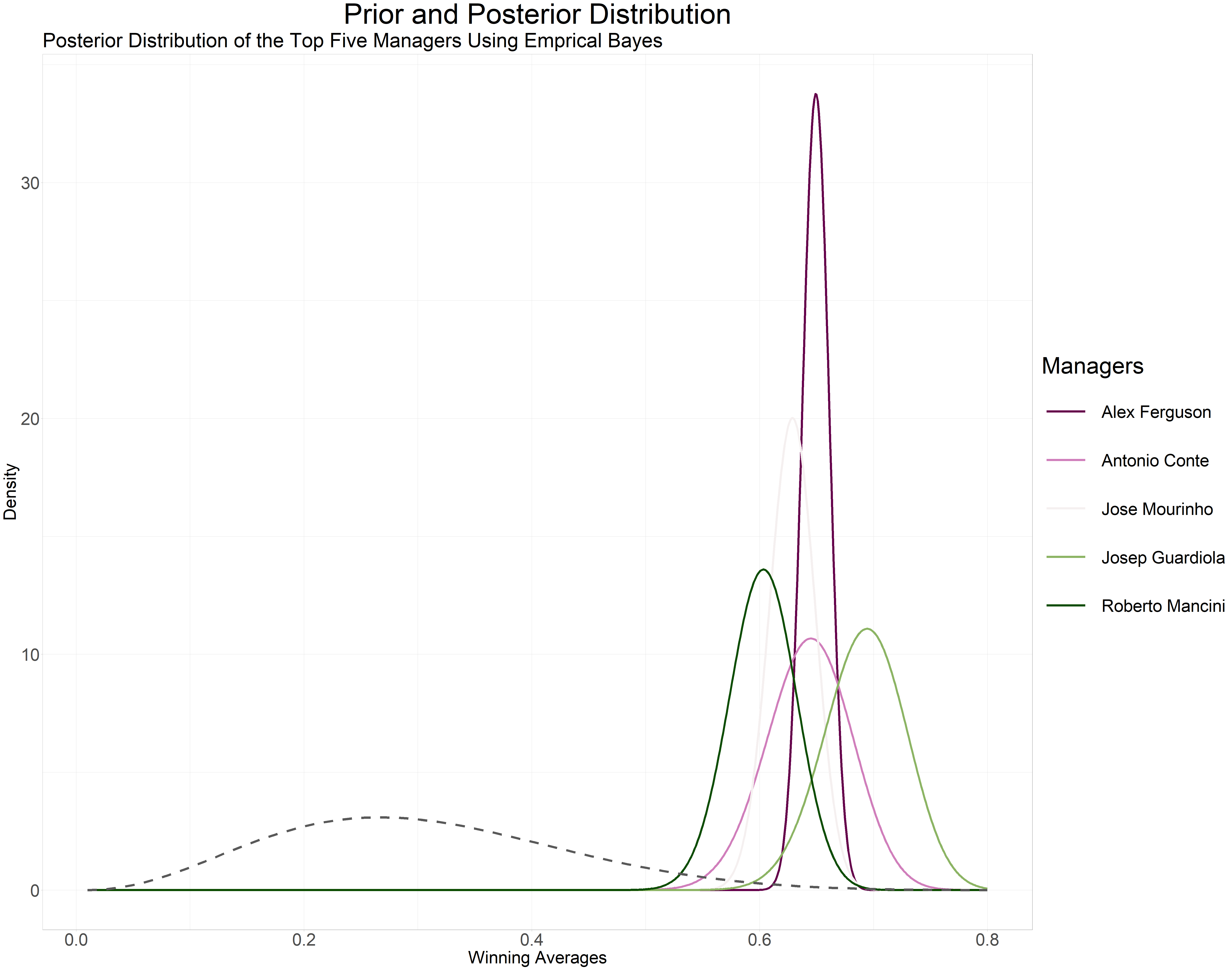
Now that we have the $$\alpha$$ and $$\beta$$ for each manager we can now visualize their posterior probability distribution. We will begin by looking at the posterior probability distribution of the top 5 managers based on our empirical Bayes estimation.
epl_man4 <- epl %>%
  arrange(desc(eb_winning_average)) %>%
  top_n(5, eb_winning_average) %>%
  crossing(x = seq(0.01, 0.8, 0.001))%>%
  ungroup()%>%
  mutate(density = dbeta(x, games_won + alpha2,
         total_games_managed - games_won + beta2))

epl_man4%>%
  ggplot(aes(x, density, colour = managers)) +
  geom_line(linewidth = 1.8) +
  stat_function(fun=function(x) dbeta(x, alpha, beta), lty = 2, colour = "grey35", linewidth = 2) +
  scale_colour_scico_d(palette = "bam") +
  labs(x = "Winning Averages",
       y = "Density",
       title="Prior and Posterior Distribution",
       subtitle="Posterior Distribution of the Top Five Managers Using Emprical Bayes",
       colour = "Managers") +
  theme(plot.title = element_text(hjust = 0.5, size = 50),
        plot.subtitle = element_text(size = 35),
        axis.title = element_text(size = 30),
        axis.text = element_text(size = 30),
        legend.title = element_text(size = 40),
        legend.key.size  = unit(3, "cm"),
        legend.text = element_text(size = 30))
Sir Alex Ferguson has a narrower posterior probability distribution (since he managed more games, we have enough evidence) compared to the broader posterior probability distribution of Josep Guardiola and Antonio Conte (both managed fewer games than Sir Ferguson). The dashed curve is the prior distribution.
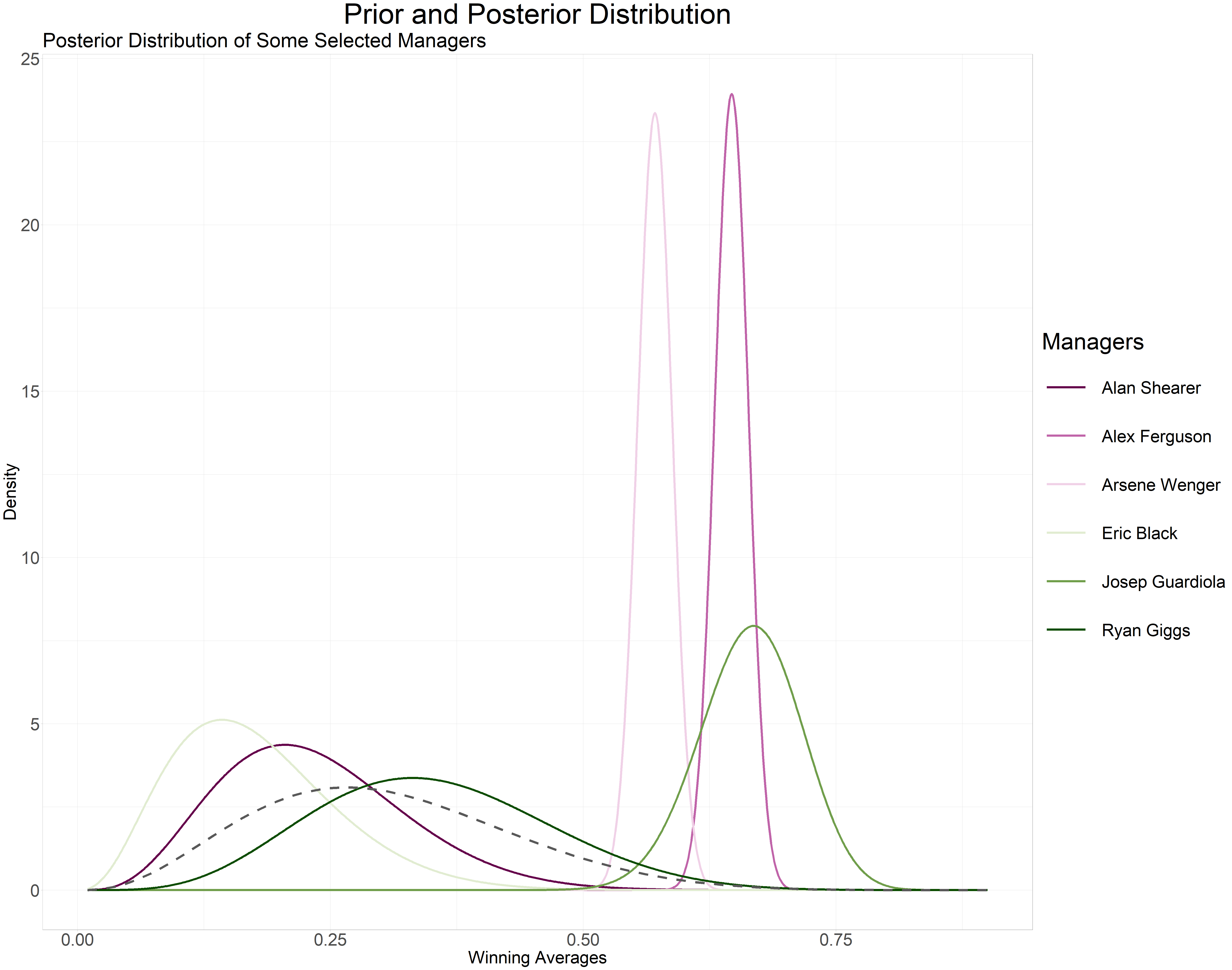
Just for fun lets compare the posterior probability distribution of a few managers outside the top 5.
manager <- c("Arsene Wenger", "Alex Ferguson", "Ryan Giggs", "Josep Guardiola", "Eric Black", "Alan Shearer")

manager_career <- epl %>%
  filter(managers %in% manager)

manager <- manager_career %>%
  crossing(x= seq(0.01, 0.9, 0.001)) %>%
  ungroup() %>%
  mutate(density = dbeta(x, alpha2, beta2))


manager%>%
  ggplot(aes(x, density, colour = managers)) +
  geom_line(linewidth = 1.8) +
  stat_function(fun=function(x) dbeta(x, alpha, beta), lty =2, colour="grey35", linewidth = 2) +
  scale_colour_scico_d(palette = "bam") +
  labs(x ="Winning Averages",
       y = "Density",
       title = "Prior and Posterior Distribution",
       subtitle="Posterior Distribution of Some Selected Managers",
       colour = "Managers") +
  theme(plot.title = element_text(hjust = 0.5, size = 50),
        plot.subtitle = element_text(size = 35),
        axis.title = element_text(size = 30),
        axis.text = element_text(size = 30),
        legend.title = element_text(size = 40),
        legend.key.size  = unit(3, "cm"),
        legend.text = element_text(size = 30))
Empirical Bayes Estimste vs Raw Average
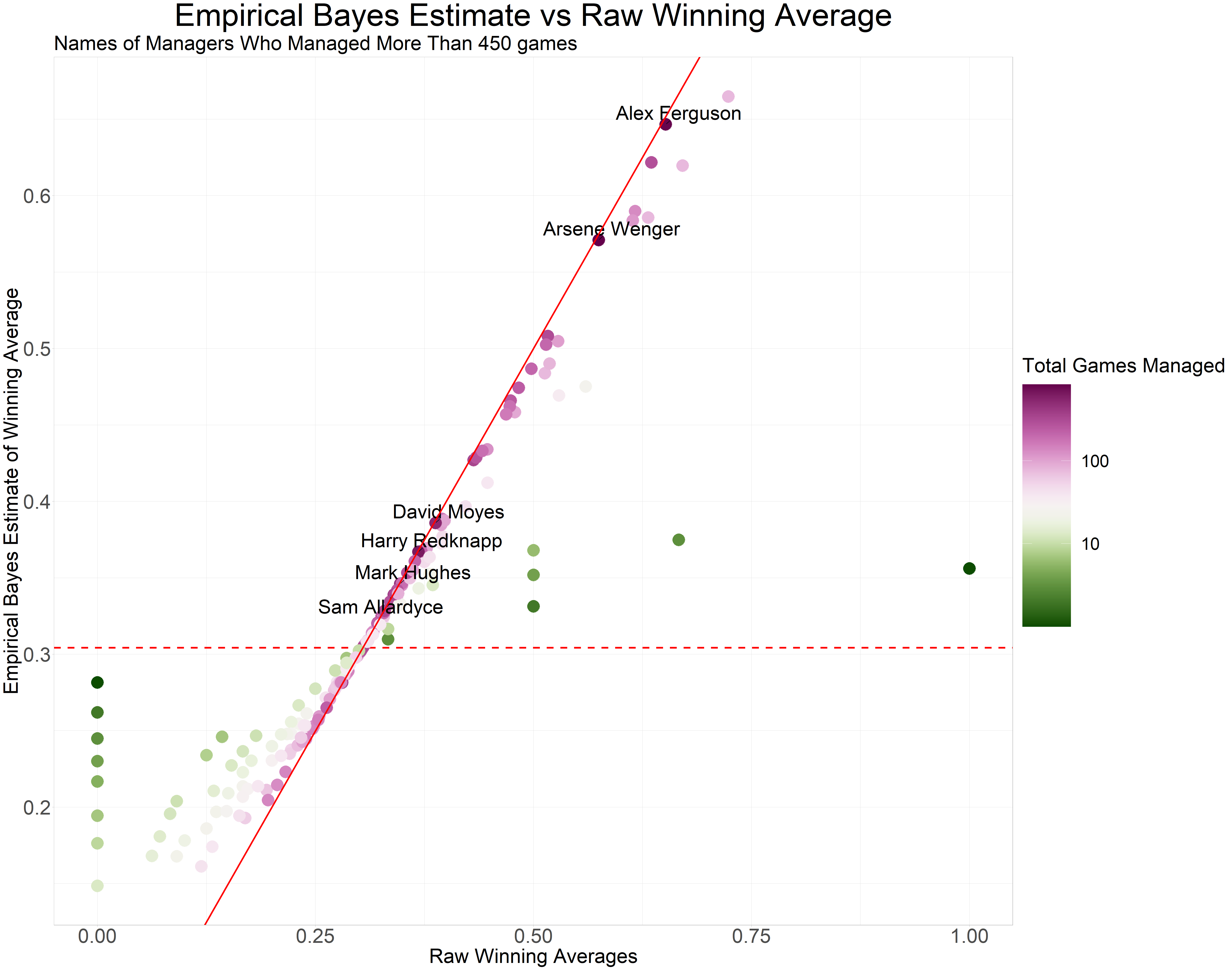
How did our empirical Bayes winning average change compared to the raw winning average? Let’s make another plot. The red dashed horizontal line marks $$y=\frac{\alpha}{\alpha + \beta}$$ this shows what each manager’s estimate would be if we had no evidence. Points above and below the line move towards this line. The diagonal line marks $$x=y$$. Points close to the line are estimates that didn’t get shrunk by empirical Bayes because we have enough evidence so their values are close to the raw estimate and they are managers that over saw more than 300 games.
library(ggrepel)

epl%>%
  ggplot(aes(average, eb_winning_average, colour = total_games_managed)) +
  geom_hline(yintercept = alpha/(alpha + beta), colour=  "red", lty=2, linewidth = 1.5)  +
  geom_point(size = 10) +
  geom_text_repel(data = subset(epl, total_games_managed >= 450), aes(label = managers), box.padding=unit(0.5, "lines"), colour="black", size = 12) +
  geom_abline(colour = "red", linetype = 1, linewidth = 1.5) +
  #scale_color_gradient(trans= "log", low="midnightblue", high="pink", name="Games Managed", breaks = 10^(1:5)) +
  scale_colour_scico(palette = "bam", trans = "log", breaks = 10^(1:5), direction = -1) +
  labs(x = "Raw Winning Averages",
       y = "Empirical Bayes Estimate of Winning Average",
       title = "Empirical Bayes Estimate vs Raw Winning Average",
       subtitle = "Names of Managers Who Managed More Than 450 games",
       colour = "Total Games Managed") +
 theme(plot.title = element_text(hjust = 0.5, size = 55),
        plot.subtitle = element_text(size = 35),
        axis.title = element_text(size = 35),
        axis.text = element_text(size = 35),
        legend.title = element_text(size = 35),
        legend.key.size  = unit(3, "cm"),
        legend.text = element_text(size = 30))
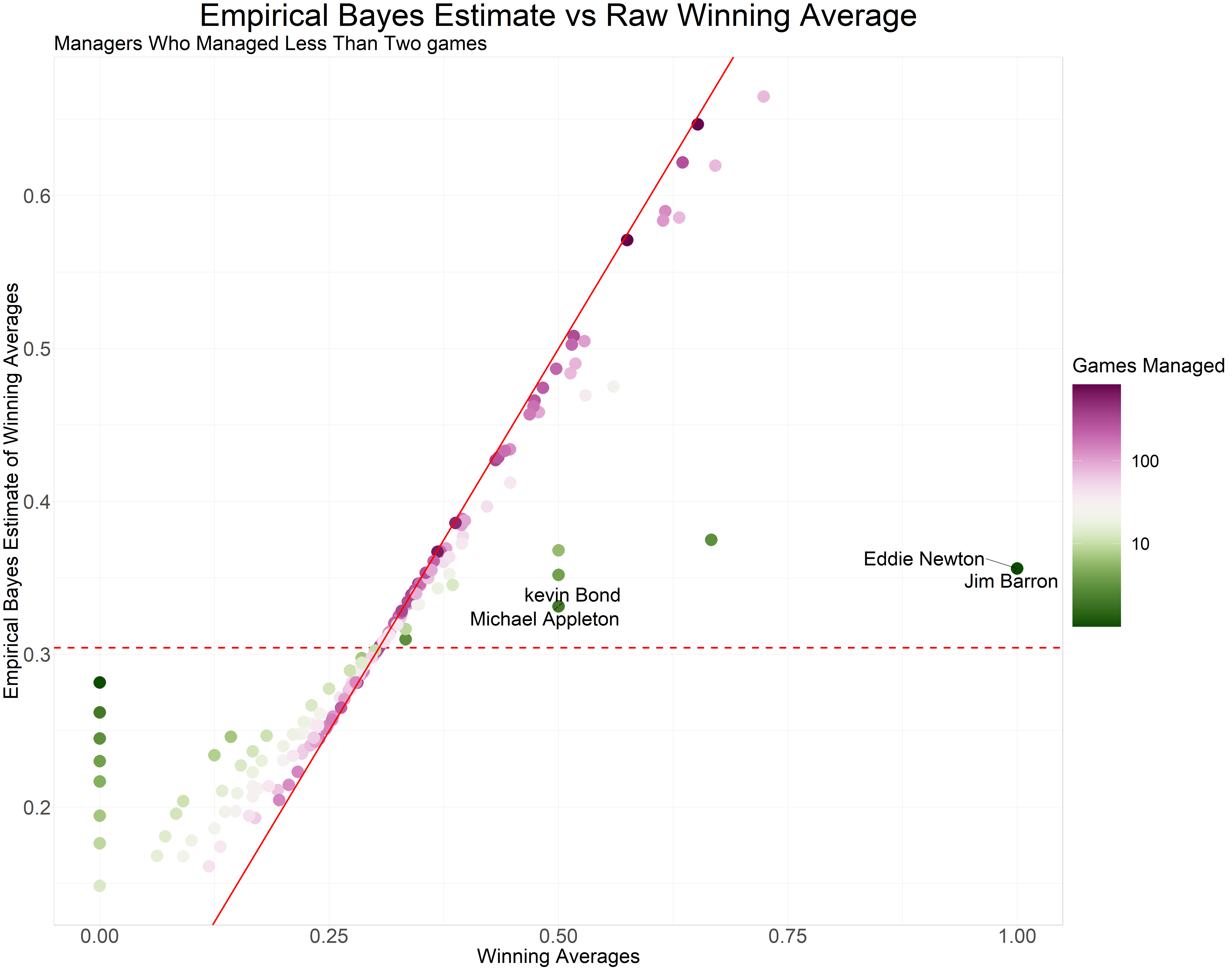
The estimates are only different for managers who over saw fewer games (less than 2 games). The raw winning average is 0 or 1 for such managers however, the empirical Bayes estimate for such managers are close to the overall mean of the prior beta distribution. This is known as shrinkage.
epl%>%
  ggplot(aes(average, eb_winning_average, colour = total_games_managed)) +
  geom_hline(yintercept = alpha/(alpha + beta), colour=  "red", lty=2, linewidth = 1.5)  +
  geom_point(size = 10) +
  geom_text_repel(data=subset(epl, total_games_managed <= 2), aes(label =  managers, colour="grey50"), box.padding = unit(0.5, "lines"), force=1.9, colour="black", size= 12) +
  geom_abline(colour = "red", linetype=1, linewidth = 1.5) +
 # scale_color_gradient(trans= "log", low="midnightblue", high="pink", name ="Games Managed", breaks = 10^(1:5)) +
  scale_colour_scico(palette = "bam", trans = "log", breaks = 10^(1:5), direction = -1) +
  labs(x = "Winning Averages",
       y = "Empirical Bayes Estimate of Winning Averages",
       title = "Empirical Bayes Estimate vs Raw Winning Average",
       subtitle = "Managers Who Managed Less Than Two games",
       colour = "Games Managed") +
 theme(plot.title = element_text(hjust = 0.5, size = 55),
        plot.subtitle = element_text(size = 35),
        axis.title = element_text(size = 35),
        axis.text = element_text(size = 35),
        legend.title = element_text(size = 35),
        legend.key.size  = unit(3, "cm"),
        legend.text = element_text(size = 30))
Step 4: Credible Interval
Credible interval tells what percentage (for this example 95%) of the the posterior winning average distribution lies within the interval. It shows how much uncertainty is present in our estimate. This computed using qbeta.
Table: Table 1: Credible Interval
| Managers | Games Won | Total Games Managed | Eb Winning Average | Low | High |
|---|---|---|---|---|---|
| Josep Guardiola | 55 | 76 | 0.665 | 0.632 | 0.759 |
| Alex Ferguson | 528 | 810 | 0.647 | 0.635 | 0.679 |
| Jose Mourinho | 183 | 288 | 0.622 | 0.603 | 0.676 |
| Antonio Conte | 51 | 76 | 0.620 | 0.585 | 0.717 |
| Roberto Mancini | 82 | 133 | 0.590 | 0.563 | 0.668 |
| Carlo Ancelotti | 48 | 76 | 0.586 | 0.551 | 0.686 |
| Manuel Pellegrini | 70 | 114 | 0.584 | 0.554 | 0.668 |
| Arsene Wenger | 476 | 828 | 0.571 | 0.559 | 0.604 |
| Rafael Benitez | 156 | 302 | 0.508 | 0.489 | 0.563 |
| Jurgen Klopp | 56 | 106 | 0.505 | 0.474 | 0.594 |
credible_interval <- epl%>%
  arrange(desc(eb_winning_average))%>%
  dplyr::select(managers, games_won, total_games_managed, eb_winning_average, low, high)%>%
  head(10)


knitr::kable(credible_interval, caption = "Credible Interval", col.names = str_to_title(str_replace_all(names(credible_interval), "_", " ")))
Table: Table 2: Credible Interval
| Managers | Games Won | Total Games Managed | Eb Winning Average | Low | High |
|---|---|---|---|---|---|
| Josep Guardiola | 55 | 76 | 0.665 | 0.632 | 0.759 |
| Alex Ferguson | 528 | 810 | 0.647 | 0.635 | 0.679 |
| Jose Mourinho | 183 | 288 | 0.622 | 0.603 | 0.676 |
| Antonio Conte | 51 | 76 | 0.620 | 0.585 | 0.717 |
| Roberto Mancini | 82 | 133 | 0.590 | 0.563 | 0.668 |
| Carlo Ancelotti | 48 | 76 | 0.586 | 0.551 | 0.686 |
| Manuel Pellegrini | 70 | 114 | 0.584 | 0.554 | 0.668 |
| Arsene Wenger | 476 | 828 | 0.571 | 0.559 | 0.604 |
| Rafael Benitez | 156 | 302 | 0.508 | 0.489 | 0.563 |
| Jurgen Klopp | 56 | 106 | 0.505 | 0.474 | 0.594 |
Managers in the top 20, their credible intervals are narrow. Managers such as Alex Ferguson and Arsene Wenger who have overseen over 800 games our uncertainty is low however managers such as Felipe Scolari and Guus Hiddink have a much broader credible interval as they have managed fewer games (less than 40 games). Let’s visualize this in a plot.
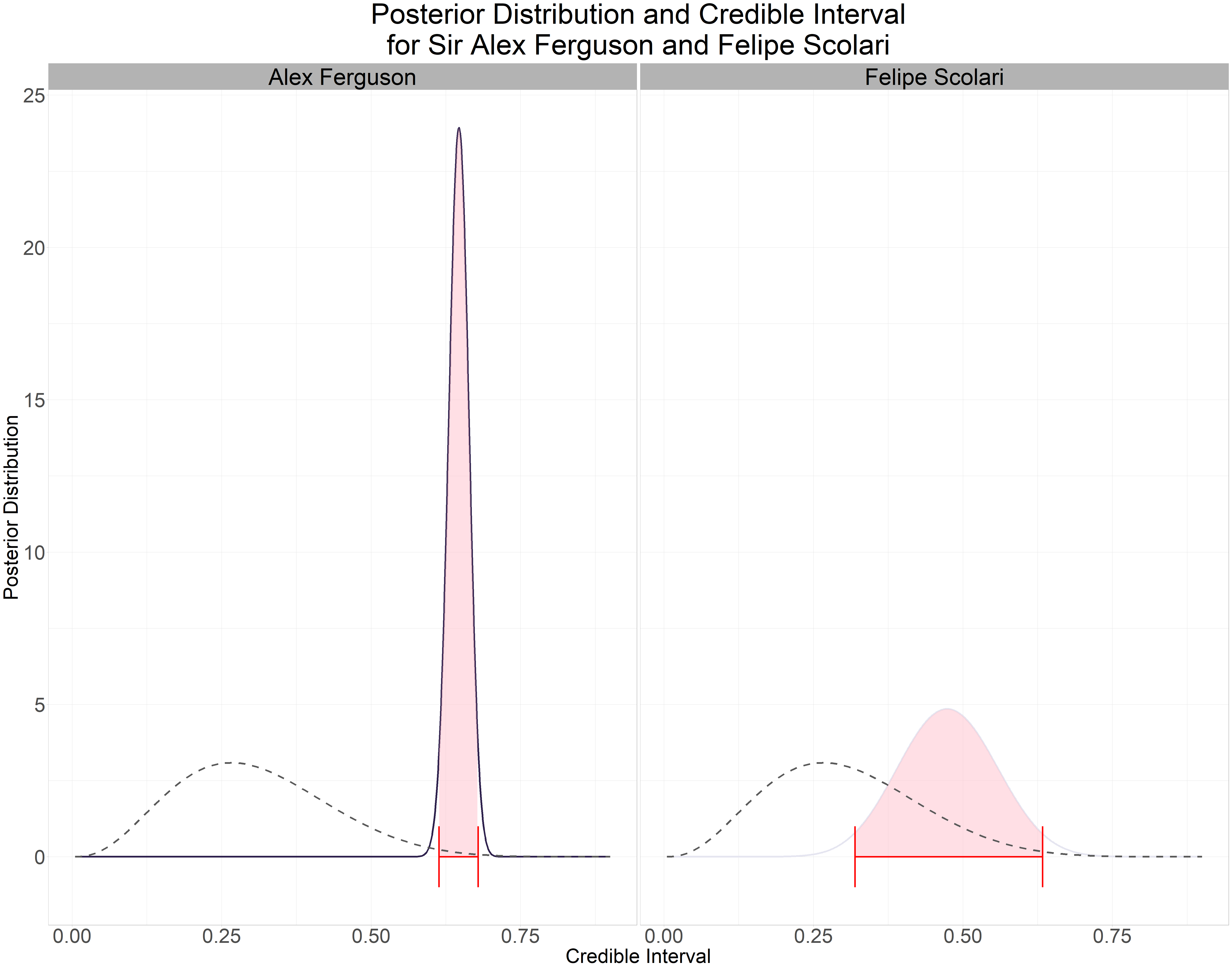
manager_ci <- c("Alex Ferguson", "Felipe Scolari")

ci <- epl %>%
  filter(managers %in% manager_ci)

ci2 <- ci %>%
  crossing(x = seq(0.005, 0.9, 0.001)) %>%
  ungroup() %>%
  mutate(density1 = dbeta(x, alpha2, beta2))


ci3 <- ci2 %>%
  mutate(cum = pbeta(x, alpha2, beta2)) %>%
  filter(cum > .025, cum < .975)


ci2 %>%
  ggplot(aes(x, density1, colour = managers)) +
  geom_line(show.legend = FALSE, linewidth = 1.5) +
  geom_ribbon(aes(ymin = 0, ymax = density1), data= ci3, alpha = 0.5, fill = "pink", show.legend = FALSE) +
  stat_function(fun=function(x) dbeta(x, alpha, beta), colour="grey35", lty=2, linewidth = 1.5) +
  geom_errorbarh(aes(xmin= qbeta(0.025, alpha2, beta2), xmax = qbeta(0.975, alpha2, beta2), y = 0), height = 2, colour = "red", linewidth = 1.3) +
  facet_wrap(~managers) +
  scale_colour_scico_d(palette = "acton") +
  labs(x = "Credible Interval",
       y = "Posterior Distribution",
       title = "Posterior Distribution and Credible Interval\nfor Sir Alex Ferguson and Felipe Scolari") +
  theme(plot.title = element_text(hjust = 0.5, size = 50),
        plot.subtitle = element_text(size = 35),
        axis.title = element_text(size = 35),
        axis.text = element_text(size = 35),
        strip.text = element_text(size = 40, colour = "black"),
        legend.title = element_text(size = 35),
        legend.key.size  = unit(3, "cm"),
        legend.text = element_text(size = 30))
Since it is difficult to visualize the credible interval and posterior probability distribution density plot for all the managers in the top 20 lets make a point and error bar plot instead.
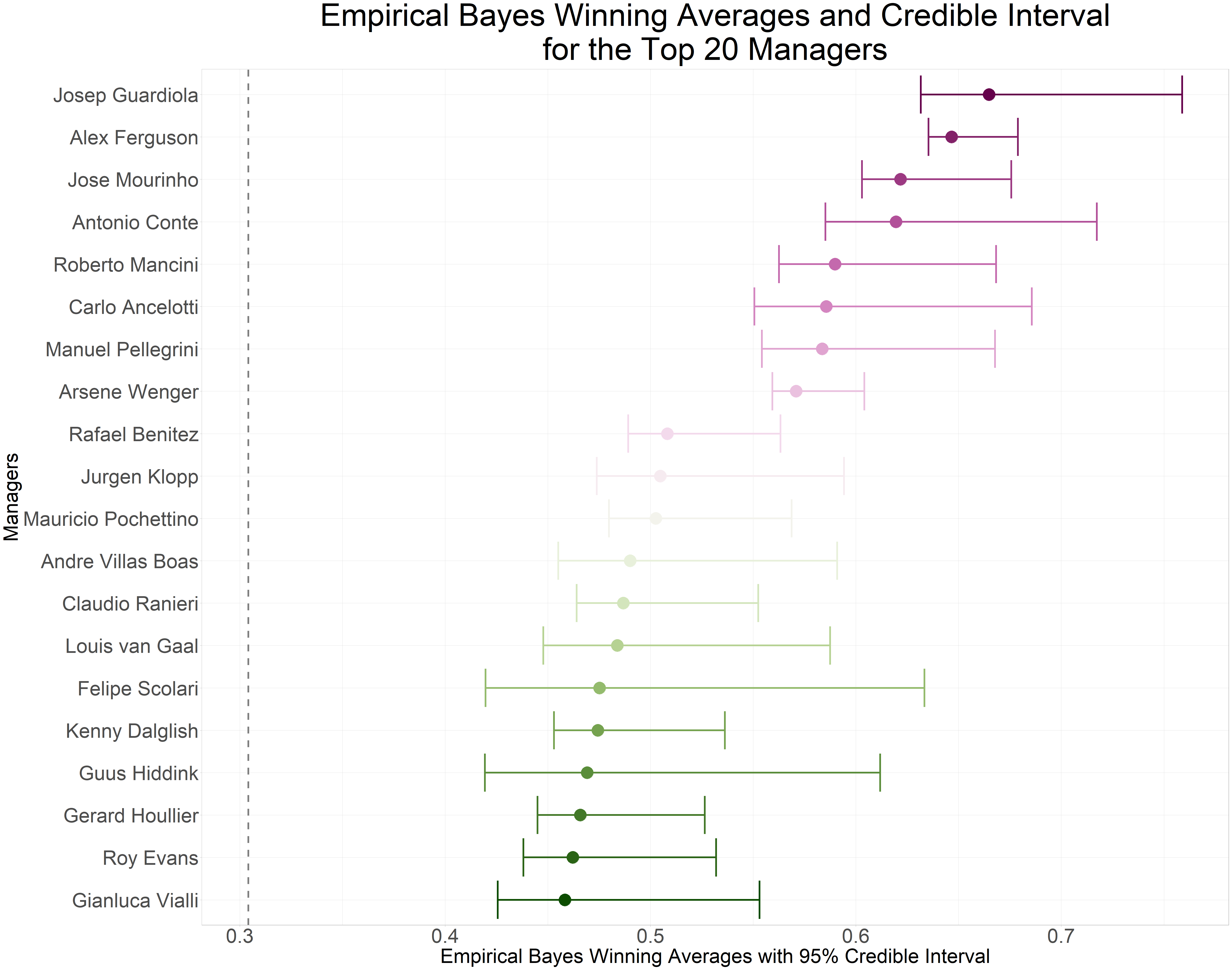
epl_man5 <- epl %>%
  arrange(desc(eb_winning_average)) %>%
  top_n(20, eb_winning_average) %>%
  mutate(managers = reorder(managers, eb_winning_average))


epl_man5%>%
  ggplot(aes(eb_winning_average, managers, colour = managers)) +
  geom_errorbarh(aes(xmin= low, xmax= high), show.legend = FALSE, linewidth = 1.5) +
  geom_point(show.legend = FALSE, size = 10) +
  geom_vline(xintercept = alpha/(alpha + beta), colour="grey50", lty=2, linewidth = 1.5)  +
  scale_colour_scico_d(palette = "bam", direction = -1) +
  labs(x = "Empirical Bayes Winning Averages with 95% Credible Interval",
       y = "Managers",
       title = "Empirical Bayes Winning Averages and Credible Interval\nfor the Top 20 Managers",
       colour = "Managers")+
  theme_light() +
  theme(plot.title = element_text(hjust = 0.5, size = 55),
        plot.subtitle = element_text(size = 35),
        axis.title = element_text(size = 35),
        axis.text = element_text(size = 35),
        legend.title = element_text(size = 35),
        legend.key.size  = unit(3, "cm"),
        legend.text = element_text(size = 30))
Appendix
During our analysis, we made several assumptions. Firstly, we assumed that all the winning averages originated from a single distribution, and secondly, we assumed that each manager managed the same team since their league debut. However, in reality, except for Alex Ferguson and Arsene Wenger who have managed only one club since their debut in the league, other managers have managed several clubs over the years, resulting in changes to their winning averages over time depending on the club they managed.
We could estimate separate beta priors for each team managed as well as for every five years.